Computational graph#
What is a computational graph?#
A computational graph is a method of representing mathematical operations using a graph structure. You can think of it as a plumbing system for data flow: data flows in from input nodes, passes through various operation nodes (such as addition, multiplication, and activation functions), and finally arrives at output nodes.
This representation offers two core values [Wer90]:
Visualization: Complex mathematical expressions become clear flowcharts
Automatic differentiation: Provides the structural foundation for backpropagation, enabling automated gradient computation
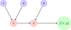
Computational graph example: \(f(x,y) = (x+y) \times y\)
In this graph:
Blue nodes: Input variables (\(x\), \(y\))
Red nodes: Operations (addition \(+\), multiplication \(\times\))
Green node: Final output
Arrows: Direction of data flow
Forward propagation: How data flows#
Forward propagation is the process where data flows from input nodes to output nodes. Following topological order (computing dependent nodes first), each operation node receives inputs and computes its output.
Example: Computing \(f(x, y, z) = (x + y) \times z\)#
Let \(x = 2\), \(y = 3\), \(z = 4\):
Input nodes: \(x = 2\), \(y = 3\), \(z = 4\)
Addition node: \(a = x + y = 2 + 3 = 5\)
Multiplication node: \(f = a \times z = 5 \times 4 = 20\)
This is the workflow of a computational graph during forward propagation.
Backpropagation: How gradients flow back#
The true power of computational graphs lies in Backpropagation Algorithm. Gradients (error signals) flow in the reverse direction along edges, propagating from output nodes back to input nodes. This enables us to efficiently compute the contribution of each parameter to the final loss.
Key insight
Computational graphs make “credit assignment” systematic:
Forward propagation: Data flows in the arrow direction to compute outputs
Backpropagation: Gradients flow in the reverse arrow direction to attribute error
Dynamic computational graphs in PyTorch#
PyTorch uses dynamic computational graphs (define-by-run): the graph is constructed dynamically during each forward pass, providing tremendous flexibility.
::
Explanation of gradient computation#
Why do gradients take these values? According to the chain rule:
\(\frac{\partial f}{\partial x} = \frac{\partial f}{\partial a} \cdot \frac{\partial a}{\partial x} = z \cdot 1 = 4\)
\(\frac{\partial f}{\partial y} = \frac{\partial f}{\partial a} \cdot \frac{\partial a}{\partial y} = z \cdot 1 = 4\)
\(\frac{\partial f}{\partial z} = a = 5\)
PyTorch’s backward() automates these calculations.
Advantages of computational graphs#
Visualizing complex computations: Deep networks can involve millions of operations; computational graphs break them down into interpretable modules.
Automatic differentiation: Eliminates manual gradient derivations; the graph structure enables automated differentiation.
Optimized execution:
By analyzing dependencies, engines can:
Determine optimal execution order
Identify parallelizable operations
Avoid redundant computations
From computational graphs to neural networks#
Computational graphs of neural networks feature:
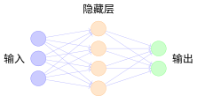
Simplified neural network computational graph
Multi-layer structure: Input layer → Hidden layer → Output layer
Weight parameters: Each edge represents a learnable weight
Activation functions: Each node typically incorporates a non-linear transformation
In the next section, we will explore Activation Functions in depth—how non-linear operations in the computational graph empower neural networks to partition complex decision boundaries.
Summary#
The Computational graph is the core data structure in deep learning:
Forward propagation: Data flows along edges to compute prediction results
Backpropagation: Gradients flow backward along edges, laying the foundation for Backpropagation Algorithm
Automatic differentiation: The graph structure automates gradient computation in Backpropagation Algorithm
Having understood Computational graph, we will explore how Activation Functions partition decision boundaries in feature space via non-linear transformations. Then Loss Functions quantify prediction errors, Backpropagation Algorithm computes gradients efficiently over the computational graph, and finally Gradient Descent and Optimization Algorithms leverages these gradients to optimize parameters.
References
Contributors and Revision History
View detailed revision history
-
e2bc8802026-06-13 - Heyan Zhu: fix: missing bib keys in pdf output -
d7c9da72026-05-12 - Heyan Zhu: docs: update sphinx only filter from not pdf to not latex -
a954ca52026-05-11 - Heyan Zhu: docs: revise and restructure documentation, fix formatting, and move env setup and sphinx guide to a separate appendix section -
f159d562026-05-08 - Heyan Zhu: fix: address complaints from the linter -
59126f42026-04-26 - Heyan Zhu: docs(math-fundamentals): update content structure and add citations -
756a7932026-04-25 - Heyan Zhu: docs(math-fundamentals): update content structure and improve explanations -
cec393d2025-12-11 - Heyan Zhu: docs: partially complete migration and restructure course materials -
0c291d72025-12-10 - Heyan Zhu: docs: restructure course materials and add new content