Learning Task Formulations

The computational graph introduced in Computational graph describes how data flows through a model. But toward what objective does the data flow? Different types of “patterns” require different mathematical modeling approaches.

What Patterns Does Machine Learning Look For?

The essence of machine learning is to discover patterns from data and then use these patterns to make predictions [Bis06]. However, “patterns” come in different forms:

Pattern Type	Core Question	Example
Category Boundaries	What common features do things of this type share?	Classifying cats and dogs
Numerical Mappings	What is the relationship between input and output?	Predicting house prices based on area
Sequence Dependencies	What should come next?	Completing a sentence

These three pattern types correspond to three task formulations: classification, regression, and autoregression. They share the same computational mechanism in the Computational graph, but their target mathematical formulations are distinctly different.

---

Classification Tasks: Discovering Category Boundary Patterns

Imagine teaching a child to recognize animals. Instead of showing them a checklist, you point at a picture and say, “This one has four legs, fur, and barks, so it’s a dog.”

Essence of Classification: Finding the boundary that separates different categories—class A on one side, class B on the other.

In feature space, each sample is a point, and classification is drawing a decision boundary that partitions the space:

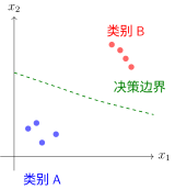
Decision Boundary in Classification Tasks

Key Insights:

• Samples of the same class cluster on one side of the boundary

• Boundaries are “soft” (probabilistic) rather than rigid hard cuts

• A new sample is predicted as whichever class its location falls into

Mathematical Formulation: A classification model outputs a class probability distribution \(p(y=k|x)\), where \(k \in \{1, 2, ..., K\}\). The decision rule selects the class with maximum probability:

\[\hat{y} = \arg\max_k \, p(y=k|x)\]

The decision boundary lies where two class probabilities are equal: \(p(y=i|x) = p(y=j|x)\).

The non-linear activation functions discussed in Activation Functions exist precisely to enable neural networks to learn non-linear decision boundaries. Without non-linear activations, no matter how many layers a network has, it can only learn linear boundaries.

---

Regression Tasks: Discovering Numerical Mapping Patterns

Imagine conducting a physics experiment measuring spring extension under different pulling forces. You observe that “the greater the force, the longer the extension.” This is not a classification problem—you are not sorting force into “large” or “small” categories, but finding a precise numerical relationship.

Essence of Regression: Learning a functional mapping that takes numerical inputs and produces numerical outputs.

The simplest form of regression is linear regression, assuming a straight-line relationship between input and output. By analogy: you collect data on house floor areas and prices, scatter-plot them on paper, and draw the line that best “fits” the points.

Mathematical Formulation: For single-variable linear regression:

\[\hat{y} = wx + b\]

• \(x\): Input feature (e.g., house floor area)

• \(w\): Weight (slope, representing “price per square meter”)

• \(b\): Bias (intercept, representing “base price”)

• \(\hat{y}\): Predicted value (predicted house price)

Geometric Interpretation

In a 2D plane, linear regression finds a straight line that minimizes the sum of vertical distances from all data points to the line.

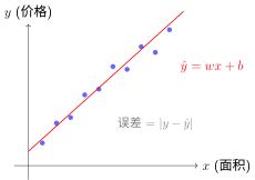
Geometric Meaning of Linear Regression

Extension to Multiple Variables: Real-world house prices depend not only on floor area, but also on location, age, floor, etc. Multivariable linear regression:

\[\hat{y} = w_1x_1 + w_2x_2 + ... + w_dx_d + b = \mathbf{w}^T\mathbf{x} + b\]

This is no longer a straight line in a 2D plane, but a hyperplane in high-dimensional space.

Non-linear Regression

Linear regression assumes a straight-line relationship, but many patterns in nature are curved. By stacking non-linear layers, neural networks can learn arbitrarily complex function mappings.

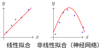
From Linear to Non-linear Regression

Fundamental Differences: Regression vs Classification

Dimension	Classification	Regression
Pattern Form	Category boundaries (partitioning regions)	Function mapping (input → output)
Output Space	Discrete finite set \(\{1,...,K\}\)	Continuous infinite set \(\mathbb{R}\)
Prediction Target	“Which category is this?”	“What is the numerical value?”
Error Metric	Classification error rate	Numerical deviation \(|y - \hat{y}|\)
Geometric Analogy	Separating surface in space	Fitted surface in space

Summary in One Sentence: Classification is “slicing a cake” (partitioning space), while regression is “drawing a curve” (fitting relationships).

---

Autoregressive Tasks: Discovering Sequence Dependency Patterns

Imagine listening to a story: “Once upon a time, there was a mountain, and in the mountain there was a…” You naturally expect “temple”. Why not “castle” or “school”? Because from experience, “temple” is the most common word following that context.

Essence of Autoregression: Predicting the next token based on already generated content, step by step.

Probability Factorization: The joint probability of a sequence can be factorized using the chain rule. For two events, \(p(A,B) = p(A) \cdot p(B|A)\)—first \(A\) occurs, then \(B\) occurs given \(A\). Extending this to sequences:

\[p(y_1, y_2, y_3) = p(y_1) \cdot p(y_2|y_1) \cdot p(y_3|y_1, y_2)\]

General form:

\[p(y_1, y_2, ..., y_T) = \prod_{t=1}^{T} p(y_t | y_{<t})\]

where \(y_{<t}\) denotes all historical content from \(y_1\) to \(y_{t-1}\).

Why is this factorization useful? Imagine generating the sentence “The cat sat on the mat”. Learning the probability of the entire sentence at once is difficult, but after factorization, every step becomes a simple classification task:

• \(p(\text{The}|\text{<s>})\): Probability of starting with “The”

• \(p(\text{cat}|\text{<s>The})\): Probability of following “The” with “cat”

• \(p(\text{sat}|\text{<s>The cat})\): Probability of following “The cat” with “sat”

Causality Constraint: Autoregression can only depend on the past, with no “peeking” into the future:

\[::\]

This is like writing an essay—you cannot use unwritten sentences to decide what to write now. This “left-only” property is called causal masking.

Training vs. Inference:

• During Training: The full sequence “The cat sat on the mat” is known, and the model learns conditional probabilities at all positions simultaneously. Losses across all positions can be computed in parallel.

• During Inference: Starting from <start>, the model generates the first word, uses it as input to generate the second word, and so on. This must proceed sequentially.

Tree Structure of Sequence Generation:

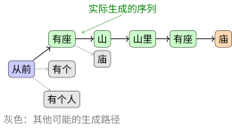
Sequence Generation in Autoregression

At each step, the model outputs a probability distribution, then samples (or selects the maximum probability token) to produce the next word.

Connection to Classification: Every step of autoregression is fundamentally classification—selecting a token from a vocabulary. The difference is that standard classification predictions are independent, whereas each autoregressive prediction depends on all historical choices—it is “classification with memory”. Evaluation also considers overall sequence quality (measured by perplexity) rather than just single-step accuracy.

---

Unification and Differences Among the Three Tasks

All three task types follow the same computational framework (see Computational graph): Input → Transformation → Output → Loss Computation. The key differences lie in output layer design and choice of loss function.

Task	Pattern Form	Output Layer	Typical Loss	Geometric Intuition
Classification	Category boundary	Softmax	Cross-entropy	Spatial region partitioning
Regression	Function mapping	Linear	MSE/MAE	Surface fitting
Autoregression	Conditional probability chain	Softmax (per step)	Cumulative cross-entropy	Tree expansion

Processing flow for the same input across different tasks:

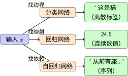
Comparison of Processing Workflows Across Three Task Types

---

Summary

Concept	Practice	Connection
Classification	Discovering category boundaries	Learn non-linear boundaries using Activation Functions
Regression	Learning function mappings	Linear regression forms the foundation; neural networks extend it to non-linearity
Autoregression	Modeling sequence dependencies	Classification at each step, building a sequence as a whole

The differences among the three task types lie not in internal network architecture (all can stack similar layers), but in:

1. Output layer design (Softmax vs. Linear vs. Per-step Softmax)

2. Choice of loss function (Cross-entropy vs. MSE vs. Cumulative cross-entropy)

3. Evaluation method (Accuracy vs. Error magnitude vs. Sequence quality)

Having understood the mathematical formulations of these three tasks, Loss Functions will cover in detail how loss functions quantify prediction quality—cross-entropy for classification, MSE for regression, and cumulative cross-entropy for autoregression. These loss functions shape different optimization surfaces for Gradient Descent and Optimization Algorithms.

---

References

[Bis06] (1,2,3)

Christopher M Bishop. Pattern recognition and machine learning. Springer, 2006.

Contributors and Revision History

View detailed revision history

• dc35df2 2026-06-14 - Heyan Zhu: refactor: unify into two-chapter mountain-climbing narrative
• e2bc880 2026-06-13 - Heyan Zhu: fix: missing bib keys in pdf output
• d7c9da7 2026-05-12 - Heyan Zhu: docs: update sphinx only filter from not pdf to not latex
• a954ca5 2026-05-11 - Heyan Zhu: docs: revise and restructure documentation, fix formatting, and move env setup and sphinx guide to a separate appendix section
• f159d56 2026-05-08 - Heyan Zhu: fix: address complaints from the linter
• 59126f4 2026-04-26 - Heyan Zhu: docs(math-fundamentals): update content structure and add citations
• ae2053f 2026-04-26 - Heyan Zhu: docs(math-fundamentals): add task-formulations and update related content