Loss Functions

In Learning Task Formulations, we discussed the mathematical formulations of classification, regression, and autoregression tasks. Different tasks require different ways to quantify “prediction quality”—which is precisely the role of loss functions.

Essence of Loss Functions: Defining the Optimization Goal

A loss function measures the discrepancy between model predictions and true targets, transforming training into an optimization problem. Different task types correspond to different loss functions, shaping distinct loss surface geometries that affect the difficulty of optimization via Gradient Descent and Optimization Algorithms.

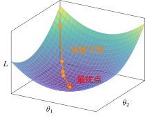
Loss Functions Define Error Surfaces

Core Roles:

• Quantifying error: Converts prediction quality into a computable numeric value

• Guiding optimization: Instructs the model “how to adjust” via gradients (see Gradient Descent and Optimization Algorithms for details)

• Shaping the landscape: Different loss functions correspond to different optimization difficulties for Gradient Descent and Optimization Algorithms

---

Loss Functions for Regression Problems

Mean Squared Error (MSE)

“Zero Tolerance” for Large Errors

Imagine playing darts. If you throw very close to the bullseye, the error is small, which is fine. But if you miss by a wide margin, squared error makes this mistake look exceptionally large—much like a teacher deducting 1 point for a minor error but 10 points for a major blunder.

Why square? Because squaring amplifies large deviations. When the error is 2, the penalty is 4; when the error is 4, the penalty jumps to 16. This “zero tolerance for large errors” property causes the model to focus heavily on samples with wildly inaccurate predictions.

Cost: Excessive sensitivity to outliers. If an extreme outlier exists in the dataset, MSE will sacrifice accuracy across most normal samples just to appease that single outlier.

Mathematical Form

\[\text{MSE} = \frac{1}{n} \sum_{i=1}^n (y_i - \hat{y}_i)^2\]

Characteristics:

• Heavier penalty on large errors (quadratic growth)

• Everywhere differentiable, facilitating gradient computation

• Sensitive to outliers

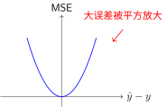
Shape of the MSE Loss Function

Mean Absolute Error (MAE)

“Fair Referee” Treating All Errors Equally

MSE acts like a strict teacher—deducting few points for small mistakes but harsh penalties for big ones. MAE, on the other hand, acts like a fair referee: deducting 1 point for a deviation of 1, and 10 points for a deviation of 10, treating all deviations equally.

Advantage: Robust against individual extreme values. If noisy points or outliers exist in the data (such as a 1-billion-dollar mansion mixed into house price data), MAE will not sacrifice prediction accuracy on typical homes just to fit that single outlier.

Cost: Non-differentiable at zero error (forming a sharp V-shape rather than a smooth curve), making optimization slightly more involved. Furthermore, because it treats all errors equally, penalty on small errors is relatively mild, resulting in potentially slower convergence than MSE.

\[\text{MAE} = \frac{1}{n} \sum_{i=1}^n |y_i - \hat{y}_i|\]

Characteristics:

• More robust to outliers (linear penalty)

• Non-differentiable at zero (subgradient available)

Huber Loss (Smooth L1)

A Piecewise Compromise

Huber loss [Hub64] is like a wise teacher who tailors guidance to circumstance:

• For small errors (\(|\text{error}| \le \delta\)): Strict like MSE—quadratic penalty keeps the model sensitive to small errors for fast convergence.

• For large errors (\(|\text{error}| > \delta\)): Rational like MAE—linear penalty prevents extreme outliers from dominating training gradients.

Role of parameter \(\delta\): Establishes a threshold (“red line”). Errors within \(\delta\) use quadratic penalty (strict), while errors beyond \(\delta\) switch to linear penalty (tolerant). Object detection tasks commonly use Huber loss because small bounding box errors demand precise localization, whereas large errors might reflect annotation noise that should not overwhelm training.

Mathematical Form

\[\begin{split}L_\delta(a) = \begin{cases} \frac{1}{2}a^2 & |a| \leq \delta \\ \delta(|a| - \frac{1}{2}\delta) & \text{otherwise} \end{cases}\end{split}\]

Characteristics:

• Small errors: MSE (smooth)

• Large errors: MAE (robust)

• Commonly used in object detection and related tasks

---

Loss Functions for Classification Problems

Cross-Entropy Loss

Understanding from an Information Coding Perspective

Imagine transmitting a message: “This is a picture of a cat.” If there are only 10 possible classes, the most straightforward encoding is assigning an integer ID (0–9). But this approach has a flaw: if the model predicts an 80% probability for “dog” and 20% for “cat”, integer IDs discard all confidence information.

A better approach uses a probability distribution as code, where model outputs like \([0.1, 0.7, 0.05, ...]\) express confidence across classes.

One-Hot Encoding: Converts categorical labels into vectors where the target class position is 1 and all others are 0.

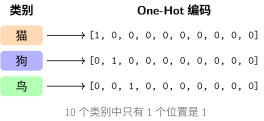
Example of One-Hot Encoding

Why is it called “One-Hot”?

• One: Exactly one position contains a 1

• Hot: That single position is “active” (hot), while all others are “cold” (0)

Cross-Entropy Formula

Cross-entropy measures the average code length required when encoding true distribution \(P\) using predicted distribution \(Q\):

\[\text{CE}(P, Q) = -\sum_{i} P(i) \log Q(i)\]

For classification problems (where \(P\) is one-hot encoded), this simplifies to:

\[::\]

Key Properties:

• More accurate predictions (probability closer to 1) yield lower loss

• Heavy penalty for incorrect predictions (loss \(\to \infty\) as predicted probability \(\to 0\))

• Yields a remarkably clean gradient when combined with Softmax

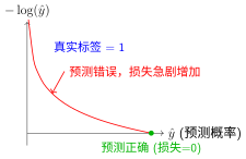
Cross-Entropy Loss: Penalizing Confident Wrong Predictions

Why not use MSE for classification?

• MSE yields tiny gradients when predicted probabilities approach 0 or 1, slowing down learning

• Cross-entropy provides much stronger gradient signals during confident mispredictions

KL Divergence (Kullback-Leibler Divergence)

Intuition: Extra Coding Penalty

Imagine you have a perfect weather forecasting model \(P\) (knowing the actual daily probability of rain), but you must use another model \(Q\) for predictions. KL divergence measures how much extra information you need to transmit because you used imperfect model \(Q\) instead of true distribution \(P\).

\[D_{KL}(P \| Q) = \sum_{i} P(i) \log \frac{P(i)}{Q(i)}\]

Intuitive Examples:

• If \(Q = P\) (perfect prediction), the extra cost is 0

• If predictions are frequently wrong, the extra cost is high

• Asymmetric: Cost of approximating \(P\) with \(Q\) \(\neq\) cost of approximating \(Q\) with \(P\)

Relationship to Cross-Entropy

\[::\]

where \(H(P)\) is the entropy of distribution \(P\) (the minimum possible code length in information theory). Since the ground-truth distribution \(P\) is fixed, \(H(P)\) is constant. Therefore:

Minimizing Cross-Entropy = Minimizing KL Divergence = Driving predicted distribution as close as possible to the true distribution

Application Scenarios

• Variational Autoencoders (VAEs): Constraining the latent distribution \(z\) to match a standard normal distribution

• Knowledge Distillation: Teaching a small model to match the “soft predictions” (probability distributions) of a teacher model rather than hard labels

• Reinforcement Learning: Constraining policy update step sizes to prevent drastic policy drift

---

Loss Function Selection Guide

Reference for Selecting Loss Functions

Problem Type	Recommended Loss	Advantages	Caveats
Regression problem	MSE / MAE	MSE is smooth and differentiable; MAE is robust	Choose MAE when dataset contains outliers
Regression (demanding robustness)	Huber loss	Combines benefits of both MSE and MAE	Requires tuning hyperparameter \(\delta\)
Binary classification	Binary cross-entropy	Strong gradients, fast convergence	Requires Sigmoid activation on output
Multi-class classification	Cross-entropy	Best performance when paired with Softmax	PyTorch’s CrossEntropyLoss integrates Softmax
Distribution matching	KL divergence	Measures distribution discrepancy	Mind asymmetry direction \(P \| Q\)

---

PyTorch Implementation Example

::

---

Summary

Loss functions define “what makes a good prediction”, converting training into an optimization problem:

1. Regression problems: MSE is smooth and easy to optimize; MAE is robust against outliers

2. Classification problems: Cross-entropy provides strong gradients and is the mainstream choice in deep learning

3. Distribution matching: KL divergence measures probability distribution discrepancies, serving as a core tool in VAEs and knowledge distillation

Having understood loss functions, we will explore Backpropagation Algorithm—how to efficiently compute gradients and perform error “credit assignment”.

---

References

[Hub64] (1,2,3)

Peter J Huber. Robust estimation of a location parameter. The Annals of Mathematical Statistics, 35(1):73–101, 1964.

Contributors and Revision History

View detailed revision history

• e2bc880 2026-06-13 - Heyan Zhu: fix: missing bib keys in pdf output
• d7c9da7 2026-05-12 - Heyan Zhu: docs: update sphinx only filter from not pdf to not latex
• a954ca5 2026-05-11 - Heyan Zhu: docs: revise and restructure documentation, fix formatting, and move env setup and sphinx guide to a separate appendix section
• f159d56 2026-05-08 - Heyan Zhu: fix: address complaints from the linter
• 59126f4 2026-04-26 - Heyan Zhu: docs(math-fundamentals): update content structure and add citations
• ae2053f 2026-04-26 - Heyan Zhu: docs(math-fundamentals): add task-formulations and update related content
• 756a793 2026-04-25 - Heyan Zhu: docs(math-fundamentals): update content structure and improve explanations
• dcecce4 2026-01-26 - Heyan Zhu: docs: enrich math fundamentals documentation with code captions and TikZ visualizations
• 0c291d7 2025-12-10 - Heyan Zhu: docs: restructure course materials and add new content