Gradient Descent and Optimization Algorithms

Descending a Mountain Along the Steepest Direction

Imagine you are lost on a mountain and want to descend to the valley:

• Current position: current parameter value \(\theta_t\)

• Steepest descent direction: negative gradient direction (the steepest downhill direction under your feet)

• Step size: learning rate \(\eta\) (how large a step you take)

• Goal: reach the bottom of the valley (minimum loss \(L\))

Once neural network training is formulated as an optimization problem, we need to find the minimum point of the loss function. Gradient descent is the iterative algorithm used to solve this problem.

Core idea: At the current position, take a small step along the direction of gradient descent (the direction in which loss decreases fastest).

\[ \theta_{t+1} = \theta_t - \eta \cdot \nabla_\theta J(\theta) \]

where \(\eta\) is the learning rate (step size), and \(\nabla_\theta J(\theta)\) is the gradient of the loss function with respect to the parameters.

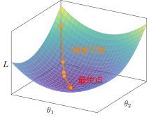
Gradient Descent: Gradually Approaching the Minimum from the Initial Point

Importance of the Learning Rate

The choice of learning rate is critical:

Learning Rate	Effect	Analogy
Too small	Extremely slow convergence	Baby steps
Appropriate	Fast convergence	Normal walking
Too large	Oscillation / divergence	Giant leap, may overshoot the valley

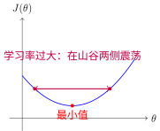
Learning Rate Too Large Causing Oscillation

---

Variants of Gradient Descent

In Gradient Descent and Optimization Algorithms, we update parameters based on the gradients computed by Backpropagation Algorithm. Depending on how much data is used to compute the gradient, there are three variants:

Batch Gradient Descent (Batch GD)

Computes gradients using all data:

\[ \theta_{t+1} = \theta_t - \eta \cdot \frac{1}{N} \sum_{i=1}^N \nabla_\theta J(\theta; x_i, y_i) \]

Characteristics:

• Accurate gradient estimation, stable convergence

• High computational cost per iteration, unsuitable for large datasets

Stochastic Gradient Descent (SGD)

Computes gradients using a single sample at each step:

\[ \theta_{t+1} = \theta_t - \eta \cdot \nabla_\theta J(\theta; x_i, y_i) \]

Characteristics:

• Fast computation, suitable for online learning

• Noisy gradients, unstable convergence

• Noise may help escape local optima

Mini-batch Gradient Descent (Mini-batch GD)

Computes gradients using a mini-batch of samples (typically 32–256):

\[ \theta_{t+1} = \theta_t - \eta \cdot \frac{1}{m} \sum_{i=1}^m \nabla_\theta J(\theta; x_i, y_i) \]

Characteristics:

• Balances computational efficiency and stability

• Can leverage GPU parallel computing

• Most commonly used in deep learning

---

Advanced Optimization Algorithms

Loss Landscape: Optimization Terrain Shaped by Loss Functions

The Loss Landscape describes the shape of Loss Functions in parameter space. Imagine a high-dimensional mountainous terrain: valleys represent regions of low loss, while peaks represent regions of high loss.

In deep learning, this landscape is usually non-convex, containing:

• Local optima: local valleys (shallow pits)

• Global optimum: the deepest valley (the optimal solution)

• Saddle points: saddle-shaped points (very common in high-dimensional spaces)

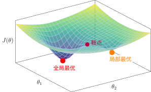
Loss Landscape: Local Optima vs. Global Optimum

Key Observations:

• The global optimum is significantly deeper than the local optimum (the red point is far below the orange point)

• The two optima are separated by a saddle point (purple)

• Optimization algorithms need to “cross over” saddle points to move from a local optimum to the global optimum

Detailed View of Saddle Points:

A saddle point resembles a horse saddle—it is a minimum along one direction and a maximum along another:

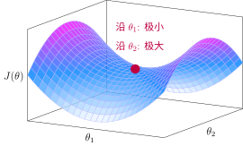
Saddle Point: Saddle Shape

Special Circumstances in Deep Learning:

• In high-dimensional spaces, saddle points are much more common than local optima

• Noise in stochastic gradient descent helps escape local optima and saddle points

• Modern networks usually find good enough solutions even if they are not globally optimal

Momentum: Accumulating Velocity to Overcome Obstacles

Intuition: Imagine rolling a snowball down a hill; it accumulates momentum, rolls faster and faster, and can roll over small potholes. In a loss landscape, momentum helps us push through saddle points and flat regions.

Principle: Introduce a velocity variable to accumulate historical gradients:

\[\begin{split} \begin{aligned} v_{t+1} &= \gamma v_t + \nabla_\theta J(\theta_t) \\ \theta_{t+1} &= \theta_t - \eta \cdot v_{t+1} \end{aligned} \end{split}\]

Understanding Momentum Step by Step:

Step 1: Understand the velocity variable \(v_t\)

In standard SGD, we update parameters directly using the gradient: $\(\theta_{t+1} = \theta_t - \eta \cdot \nabla_\theta J(\theta_t)\)$

This is equivalent to completely re-deciding the direction at every step, without remembering the path taken previously.

Momentum introduces a velocity variable \(v_t\), effectively adding a “memory” to the optimization process—remembering previously accumulated movement trends.

Step 2: Interpret the velocity update formula

\[v_{t+1} = \gamma v_t + \nabla_\theta J(\theta_t)\]

This formula means: New velocity = Retained old velocity + Current gradient

Formula Details:

Symbol	Meaning	Dimension	Intuitive Understanding
\(v_{t+1}\)	Velocity at step \(t+1\)	Same as parameters	“Step vector” to be taken in the next step
\(\gamma\)	Momentum coefficient	Scalar (0–1)	Magnitude of inertia, typically 0.9 (retaining 90% of old velocity)
\(v_t\)	Velocity at step \(t\)	Same as parameters	Previously accumulated movement trend
\(\nabla_\theta J(\theta_t)\)	Current gradient	Same as parameters	Steepest descent direction at the current position

Core Insights:

• \(\gamma = 0\) (no momentum): \(v_{t+1} = \nabla_\theta J\), degenerates to basic SGD

• \(\gamma = 0.9\) (with momentum): New velocity = 90% old velocity + 10% new gradient

Step 3: Interpret the parameter update formula

\[\theta_{t+1} = \theta_t - \eta \cdot v_{t+1}\]

Difference from SGD:

• SGD: \(\theta_{t+1} = \theta_t - \eta \cdot \nabla_\theta J\) (uses only current gradient)

• Momentum: \(\theta_{t+1} = \theta_t - \eta \cdot v_{t+1}\) (uses accumulated velocity)

Why does this reduce oscillation?

Imagine walking in a ravine:

• SGD: Looking only at your feet each step, taking a step left, finding the right side lower, taking a step right, oscillating back and forth across the ravine walls

• Momentum: With inertia, walking left accumulates leftward velocity. Even if the right side is slightly lower, inertia carries you forward leftward until the left side becomes significantly higher than the right, at which point it gradually turns

Expanding the Formula to See the Essence:

If we expand the recursive definition of \(v_t\):

\[\begin{split} \begin{aligned} v_t &= \gamma v_{t-1} + g_t \\ &= \gamma (\gamma v_{t-2} + g_{t-1}) + g_t \\ &= \gamma^2 v_{t-2} + \gamma g_{t-1} + g_t \\ &= \ldots \\ &= \sum_{i=0}^{t} \gamma^{t-i} g_i \end{aligned} \end{split}\]

where \(g_i = \nabla_\theta J(\theta_i)\) is the gradient at step \(i\).

Key Finding: Current velocity is a weighted average of historical gradients, where earlier gradients have smaller weights (exponentially decaying by \(\gamma^k\)).

Analogy:

• Standard SGD: Re-decides direction at every step, making it easy to oscillate back and forth across ravine walls

• Momentum: Like a ball rolling down a hill, possessing inertia; accelerates in consistent directions and decelerates when directions reverse, naturally reducing oscillation

Effects:

• Accelerates convergence (especially when gradient directions are consistent)

• Reduces oscillation (momentum cancels out when gradient directions change)

• Helps escape local optima

Adam (Adaptive Moment Estimation)

Adam [KB15] is currently one of the most widely used optimization algorithms, combining the advantages of Momentum and RMSprop.

Intuition: Adjust the learning rate individually for each parameter. Parameters updated frequently receive smaller learning rates, while sparsely updated parameters receive larger learning rates.

Principle: Combine first-moment estimation (momentum) and second-moment estimation (adaptive learning rate):

\[\begin{split} \begin{aligned} m_t &= \beta_1 m_{t-1} + (1-\beta_1) g_t \\ v_t &= \beta_2 v_{t-1} + (1-\beta_2) g_t^2 \\ \hat{m}_t &= \frac{m_t}{1-\beta_1^t}, \quad \hat{v}_t = \frac{v_t}{1-\beta_2^t} \\ \theta_{t+1} &= \theta_t - \eta \cdot \frac{\hat{m}_t}{\sqrt{\hat{v}_t} + \epsilon} \end{aligned} \end{split}\]

Understanding Adam Step by Step:

Step 1: First-moment estimation (momentum part)

\[m_t = \beta_1 m_{t-1} + (1-\beta_1) g_t\]

Similar to momentum, this computes the exponential moving average of gradients:

Symbol	Meaning	Dimension	Intuitive Understanding
\(m_t\)	First moment (mean) at step \(t\)	Same as parameters	“Average trend” of gradients, smoothed gradient direction
\(\beta_1\)	First-moment decay rate	Scalar (0–1)	Typically 0.9, retaining 90% of historical information
\(m_{t-1}\)	First moment from the previous step	Same as parameters	Previously accumulated gradient trend
\(g_t\)	Current gradient	Same as parameters	Currently computed gradient value
\((1-\beta_1)\)	Weight of the new gradient	Scalar	New gradient accounts for 10% weight

Difference from Momentum:

• Momentum: \(v_{t+1} = \gamma v_t + \nabla_\theta J\) (weight of new gradient is 1)

• Adam: \(m_t = \beta_1 m_{t-1} + (1-\beta_1) g_t\) (weight of new gradient is \(1-\beta_1\))

Adam’s form brings \(m_t\) closer to the true gradient mean (expected value).

Expanding to See the Essence:

\[m_t = (1-\beta_1) \sum_{i=1}^{t} \beta_1^{t-i} g_i\]

This is an exponentially weighted moving average of historical gradients, where more recent gradients receive larger weights.

Step 2: Second-moment estimation (adaptive learning rate part)

\[v_t = \beta_2 v_{t-1} + (1-\beta_2) g_t^2\]

Note that \(g_t^2\) here is an element-wise square:

\[g_t^2 = (g_t^{(1)})^2, (g_t^{(2)})^2, \ldots, (g_t^{(d)})^2\]

Symbol	Meaning	Dimension	Intuitive Understanding
\(v_t\)	Second moment (uncentered variance) at step \(t\)	Same as parameters	Historical average of gradient “magnitude of variation”
\(\beta_2\)	Second-moment decay rate	Scalar (0–1)	Typically 0.999, larger than \(\beta_1\)
\(g_t^2\)	Element-wise square of gradient	Same as parameters	Magnitude information of gradients

Core Insight: \(v_t\) tracks the “activity level” of each parameter’s gradient:

• Gradients consistently large → \(v_t\) is large

• Gradients consistently small → \(v_t\) is small

Why use squares?

Squaring eliminates signs (positive or negative) and retains only magnitude information. We want to know “how large” the gradients are, rather than “which direction” they point.

Step 3: Bias Correction

\[ \hat{m}_t = \frac{m_t}{1-\beta_1^t}, \quad \hat{v}_t = \frac{v_t}{1-\beta_2^t} \]

Why is correction needed?

Problem: Initially \(m_0 = 0, v_0 = 0\)

Bias in early steps:

• Step 1: \(m_1 = (1-\beta_1) g_1\), which is about \((1-\beta_1)\) times smaller than the true mean

• Step 2: \(m_2 = \beta_1(1-\beta_1)g_1 + (1-\beta_1)g_2\), still biased

Correction Principle:

• If \(m_t\) estimates \(E[g]\), then \(E[m_t] = (1-\beta_1^t) E[g]\)

• Dividing by \((1-\beta_1^t)\) yields an unbiased estimate

Symbol	Meaning	Calculation Method
\(\hat{m}_t\)	Bias-corrected first moment	\(m_t / (1-\beta_1^t)\)
\(\hat{v}_t\)	Bias-corrected second moment	\(v_t / (1-\beta_2^t)\)
\(t\)	Current timestep	Number of training iterations

Correction Effect:

• When \(t\) is small (early stage): \(1-\beta_1^t\) is small, the divisor is small, and the amplification effect is significant

• When \(t\) is large (late stage): \(\beta_1^t \approx 0\), \(1-\beta_1^t \approx 1\), almost no correction is needed

Example (\(\beta_1 = 0.9\)):

• \(t=1\): Correction factor \(1/(1-0.9) = 10\), amplified 10-fold

• \(t=10\): Correction factor \(1/(1-0.9^{10}) \approx 1.5\), amplified 1.5-fold

• \(t=100\): Correction factor \(\approx 1.0\), virtually no correction

Step 4: Parameter update (the essence of adaptive learning rates)

\[\theta_{t+1} = \theta_t - \eta \cdot \frac{\hat{m}_t}{\sqrt{\hat{v}_t} + \epsilon}\]

Element-wise interpretation:

For the \(i\)-th parameter \(\theta^{(i)}\):

\[\theta_{t+1}^{(i)} = \theta_t^{(i)} - \eta \cdot \frac{\hat{m}_t^{(i)}}{\sqrt{\hat{v}_t^{(i)}} + \epsilon}\]

Symbol	Meaning	Role
\(\hat{m}_t^{(i)}\)	Smoothed gradient for the \(i\)-th parameter	Determines update direction
\(\sqrt{\hat{v}_t^{(i)}}\)	Gradient RMS for the \(i\)-th parameter	Determines step size scaling
\(\epsilon\)	Numerical stability constant	Prevents division by zero, typically \(10^{-8}\)
\(\eta\)	Global learning rate	Overall step size control

Core Insight - Adaptive Learning Rate Mechanism:

Suppose there are two parameters:

Parameter A (large gradient fluctuations):

• Historical gradients: [10, -8, 12, -10, 9] (wild swings)

• \(\hat{m}_t \approx 2.6\) (average gradient)

• \(\hat{v}_t \approx 100\) (average squared gradient)

• \(\sqrt{\hat{v}_t} \approx 10\)

• Update step size: \(\eta \cdot 2.6 / 10 = 0.26\eta\) (step size is scaled down)

Parameter B (small gradient fluctuations):

• Historical gradients: [0.01, -0.02, 0.015, -0.01, 0.012] (minor fluctuations)

• \(\hat{m}_t \approx 0.009\) (average gradient)

• \(\hat{v}_t \approx 0.0002\) (average squared gradient)

• \(\sqrt{\hat{v}_t} \approx 0.014\)

• Update step size: \(\eta \cdot 0.009 / 0.014 = 0.64\eta\) (relatively larger step size)

Result:

• Parameters with large gradient fluctuations → step size automatically becomes smaller (cautious updates)

• Parameters with small gradient fluctuations → step size remains relatively larger (bold updates)

Why use \(\sqrt{\hat{v}_t}\) instead of \(\hat{v}_t\)?

• The dimension of squared gradient \(g_t^2\) is the square of the original gradient

• Dividing by \(\sqrt{\hat{v}_t}\) (RMS, root mean square) cancels the dimension, making the update step size match the dimension of the original gradient

• Analogy: Standard deviation \(\sigma = \sqrt{\text{variance}}\), which shares the same dimension as the original data

Hyperparameter Summary:

Parameter	Recommended Value	Role
\(\beta_1\)	0.9	First-moment decay rate, controls momentum strength
\(\beta_2\)	0.999	Second-moment decay rate, controls adaptive sensitivity
\(\epsilon\)	\(10^{-8}\)	Numerical stability
\(\eta\)	0.001 (default)	Global learning rate

Characteristics:

• Combines momentum and adaptive learning rate

• Insensitive to hyperparameters, default first choice

• Suitable for most deep learning tasks

Recommendations for Selecting Optimization Algorithms

Algorithm	Applicable Scenarios	Characteristics
SGD + Momentum	Image classification, large models	Good generalization performance, requires tuning learning rate
Adam	Default first choice, NLP, recommendation systems	Adaptive, fast convergence, easy to use
AdamW	Transformers, large models	Improved weight decay, better performance

---

Learning Rate Scheduling: Why Adjust the Learning Rate?

Core Problem

Early in training, parameters are far from optimal, requiring a large learning rate to rapidly approach the goal. Later in training, parameters are close to optimal, requiring a small learning rate for fine adjustment to avoid oscillating around the minimum.

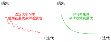
Fixed Learning Rate vs. Learning Rate Scheduling

Common Learning Rate Scheduling Strategies

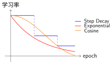
Comparison of Learning Rate Scheduling Strategies

1. 步长衰减（Step Decay）

Strategy: Multiply the learning rate by a decay factor (e.g., 0.1) every N epochs

Applicable Scenarios:

• Traditional image classification tasks (standard for ImageNet training)

• Manually reducing learning rate when validation loss stops decreasing

::

Characteristics: Stepwise reduction, simple and effective, but requires preset decay timing.

2. 指数衰减（Exponential Decay）

Strategy: Exponentially decay learning rate every epoch

\[\eta_t = \eta_0 \cdot \gamma^t\]

Applicable Scenarios:

• Smooth, continuous decay is required

• When training for a large number of epochs

::

3. 余弦退火（Cosine Annealing）

Strategy: Learning rate decays along a cosine curve from initial value to near 0

\[\eta_t = \eta_{min} + \frac{1}{2}(\eta_{max} - \eta_{min})(1 + \cos(\frac{t}{T_{max}}\pi))\]

Applicable Scenarios:

• Modern Transformer models (BERT, GPT, etc.)

• Works even better when combined with Warmup

scheduler = optim.lr_scheduler.CosineAnnealingLR(optimizer, T_max=100)

4. 预热（Warmup）

Problem: At the beginning of training, parameters are randomly initialized; gradients can be large and unstable, so a large learning rate can cause oscillation.

Strategy: Start with a very small learning rate and linearly increase it to the target learning rate.

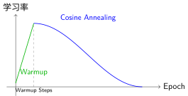
Warmup + Cosine Annealing

::

Selection Recommendations

Strategy	Recommended Scenarios	Pros	Cons
Step Decay	Image classification, CNNs	Simple and effective	Requires preset decay timing
Exponential	Long-cycle training	Smooth and continuous	Decays too quickly
Cosine	Transformers, NLP	Usually best performance	Relatively complex
Warmup + Cosine	Large model training	Stable + great performance	Requires tuning two parameters

---

PyTorch Practice

• Basic Training Loop

  ::
  

• Learning Rate Scheduling

  ::
  

---

Training Tricks

1. Gradient Clipping

   Prevents gradient exploding:

   loss.backward()
   torch.nn.utils.clip_grad_norm_(model.parameters(), max_norm=1.0)
   optimizer.step()
   

2. Batch Normalization (BatchNorm)

   Stabilizes training, accelerates convergence:

   self.bn = nn.BatchNorm1d(num_features)
   

3. Early Stopping

   Stops training when validation loss stops decreasing, preventing overfitting.

---

Summary

Gradient descent is the cornerstone of deep learning training:

1. Basic Principle: Iteratively update parameters along the negative gradient direction computed by Backpropagation Algorithm

2. Learning Rate: The most critical hyperparameter; too large causes oscillation, while too small leads to slow convergence

3. Mini-batch: Balances efficiency and stability, standard in deep learning

4. Adam: Default first-choice optimizer, adaptive and easy to use

5. Learning Rate Scheduling: Adjusting the learning rate during training improves performance

Having understood Loss Functions and optimization algorithms, you now master the full deep learning training pipeline. Next, we will review this chapter in Summary and Outlook before moving on to practical chapters.

---

References

[KB15] (1,2,3)

Diederik P Kingma and Jimmy Ba. Adam: a method for stochastic optimization. In International Conference on Learning Representations. 2015.

Contributors and Revision History

View detailed revision history

• e2bc880 2026-06-13 - Heyan Zhu: fix: missing bib keys in pdf output
• d7c9da7 2026-05-12 - Heyan Zhu: docs: update sphinx only filter from not pdf to not latex
• a954ca5 2026-05-11 - Heyan Zhu: docs: revise and restructure documentation, fix formatting, and move env setup and sphinx guide to a separate appendix section
• f159d56 2026-05-08 - Heyan Zhu: fix: address complaints from the linter
• b20ef3e 2026-04-28 - Heyan Zhu: docs: update pytorch practice section with detailed explanations and code examples
• 59126f4 2026-04-26 - Heyan Zhu: docs(math-fundamentals): update content structure and add citations
• ae2053f 2026-04-26 - Heyan Zhu: docs(math-fundamentals): add task-formulations and update related content
• 756a793 2026-04-25 - Heyan Zhu: docs(math-fundamentals): update content structure and improve explanations