神经网络模块:搭建计算图#
在 全连接神经网络 和 卷积神经网络 中,我们学习了全连接层和卷积层的数学原理:
全连接层:\(y = Wx + b\),每个输入连接所有输出
卷积层:局部感受野 + 权值共享,检测空间特征
本章将学习如何用 PyTorch 的 nn.Module 把这些数学公式变成可运行的代码。你会发现,每个层类(nn.Linear、nn.Conv2d)都直接对应一个数学运算。
从数学公式到 PyTorch 层#
全连接层:nn.Linear#
回顾 全连接神经网络:
PyTorch 实现:
import torch
import torch.nn as nn

# 输入:784维(如展平后的28×28图像)
# 输出:256维(隐藏层)
fc = nn.Linear(in_features=784, out_features=256)

# 查看参数
print(f"权重形状: {fc.weight.shape}")  # torch.Size([256, 784])
print(f"偏置形状: {fc.bias.shape}")    # torch.Size([256])

# 前向传播
x = torch.randn(64, 784)  # batch=64
y = fc(x)                 # y = x @ W^T + b
print(f"输出形状: {y.shape}")  # torch.Size([64, 256])
参数量计算
全连接层参数量 = 输入维度 × 输出维度 + 输出维度(偏置)
权重:\(784 \times 256 = 200,704\)
偏置:\(256\)
总计:200,960 参数
这与 全连接神经网络 中的计算一致。
全连接层的可视化:

全连接层结构示意图
卷积层:nn.Conv2d#
回顾 卷积神经网络:
PyTorch 实现:
# 输入:3通道图像,输出:32个特征图
# 卷积核:5×5,步长:1,填充:0
conv = nn.Conv2d(
    in_channels=3,      # 输入通道(RGB)
    out_channels=32,    # 输出通道(32个卷积核)
    kernel_size=5,      # 卷积核大小
    stride=1,           # 步长
    padding=0           # 填充
)

# 查看参数
print(f"卷积核形状: {conv.weight.shape}")  # torch.Size([32, 3, 5, 5])
print(f"偏置形状: {conv.bias.shape}")      # torch.Size([32])

# 前向传播
x = torch.randn(64, 3, 32, 32)  # batch=64, 3通道, 32×32图像
y = conv(x)                      # 卷积运算
print(f"输出形状: {y.shape}")     # torch.Size([64, 32, 28, 28])
# (32 - 5 + 0) / 1 + 1 = 28
参数量计算
卷积层参数量 = 输出通道 × 输入通道 × 卷积核高 × 卷积核宽 + 输出通道(偏置)
卷积核:\(32 \times 3 \times 5 \times 5 = 2,400\)
偏置:\(32\)
总计:2,432 参数
对比全连接层(200,960 参数),卷积层参数量少了 82 倍!这就是 归纳偏置(Inductive Bias) 的威力——利用空间局部性减少参数。
卷积层的可视化:
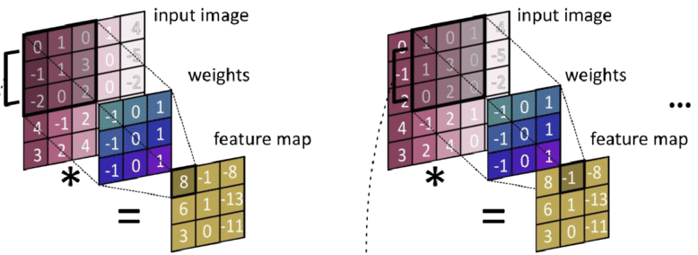
卷积运算示意图:同一个卷积核(蓝色 3×3 权重矩阵)在输入图像上滑动,每次计算点积得到一个输出值。相同的权重被共享用于检测图像不同位置的特征。#
nn.Module:构建网络的基石#
什么是 nn.Module?#
nn.Module 是 PyTorch 中所有神经网络组件的基类。它提供了:
参数管理(自动注册可学习参数)
前向传播定义(
forward方法)设备转移(
.to('cuda'))
自定义网络类#
模板:
import torch.nn as nn

class MyNetwork(nn.Module):
    def __init__(self):
        super(MyNetwork, self).__init__()

        # 1. 定义层(在__init__中创建)
        self.fc1 = nn.Linear(784, 256)
        self.relu = nn.ReLU()
        self.dropout = nn.Dropout(0.2)
        self.fc2 = nn.Linear(256, 10)

    def forward(self, x):
        # 2. 定义前向传播(数据如何流动)
        x = self.fc1(x)      # 线性变换
        x = self.relu(x)     # 激活函数(见{ref}`activation-functions`)
        x = self.dropout(x)  # 正则化(见{doc}`neural-training-basics`)
        x = self.fc2(x)      # 输出层
        return x

# 创建实例
model = MyNetwork()
print(model)
完整示例:实现 LeNet-5#
让我们用 PyTorch 实现 LeNet-5架构详解 中的经典架构:
class LeNet5(nn.Module):
    """
    LeNet-5 的 PyTorch 实现
    对应 {doc}`../neural-network-basics/le-net` 中的架构分析
    """
    def __init__(self, num_classes=10):
        super(LeNet5, self).__init__()

        # C1: 卷积层,1→6通道,5×5卷积核,输出28×28
        # 参数量: 6×1×5×5 + 6 = 156
        self.c1 = nn.Conv2d(1, 6, kernel_size=5, padding=2)

        # S2: 2×2平均池化,输出14×14
        self.s2 = nn.AvgPool2d(kernel_size=2, stride=2)

        # C3: 卷积层,6→16通道,5×5卷积核,输出10×10
        # 参数量: 16×6×5×5 + 16 = 2,416
        self.c3 = nn.Conv2d(6, 16, kernel_size=5)

        # S4: 2×2平均池化,输出5×5
        self.s4 = nn.AvgPool2d(kernel_size=2, stride=2)

        # C5: 卷积层(实为全连接),16→120,输出1×1
        # 参数量: 120×16×5×5 + 120 = 48,120
        self.c5 = nn.Conv2d(16, 120, kernel_size=5)

        # F6: 全连接层,120→84
        # 参数量: 120×84 + 84 = 10,164
        self.f6 = nn.Linear(120, 84)

        # 输出层,84→10(类别数)
        # 参数量: 84×10 + 10 = 850
        self.output = nn.Linear(84, num_classes)

    def forward(self, x):
        # C1: [batch, 1, 28, 28] → [batch, 6, 28, 28]
        x = torch.tanh(self.c1(x))

        # S2: [batch, 6, 28, 28] → [batch, 6, 14, 14]
        x = self.s2(x)

        # C3: [batch, 6, 14, 14] → [batch, 16, 10, 10]
        x = torch.tanh(self.c3(x))

        # S4: [batch, 16, 10, 10] → [batch, 16, 5, 5]
        x = self.s4(x)

        # C5: [batch, 16, 5, 5] → [batch, 120, 1, 1]
        x = torch.tanh(self.c5(x))

        # 展平: [batch, 120, 1, 1] → [batch, 120]
        x = x.view(x.size(0), -1)

        # F6: [batch, 120] → [batch, 84]
        x = torch.tanh(self.f6(x))

        # 输出: [batch, 84] → [batch, 10]
        x = self.output(x)
        return x

# 验证参数量
model = LeNet5()
total_params = sum(p.numel() for p in model.parameters())
print(f"总参数量: {total_params:,}")  # 61,706(与论文一致!)
维度追踪技巧
写 forward 时,建议在每个操作后注释输出形状:
def forward(self, x):
    x = self.conv1(x)    # [64, 3, 32, 32] → [64, 32, 28, 28]
    x = self.pool(x)     # [64, 32, 28, 28] → [64, 32, 14, 14]
    x = self.conv2(x)    # [64, 32, 14, 14] → [64, 64, 10, 10]
    # ...
这样出错时可以快速定位维度不匹配的位置。
容器:组织多个层#
nn.Sequential:顺序执行#
当层按顺序连接时,用 nn.Sequential 简化代码:
# 方式1:逐个添加
model = nn.Sequential(
    nn.Linear(784, 256),
    nn.ReLU(),
    nn.Dropout(0.2),
    nn.Linear(256, 10)
)

# 方式2:带名称(便于访问)
from collections import OrderedDict

model = nn.Sequential(OrderedDict([
    ('fc1', nn.Linear(784, 256)),
    ('relu1', nn.ReLU()),
    ('dropout', nn.Dropout(0.2)),
    ('fc2', nn.Linear(256, 10))
]))

# 访问特定层
print(model.fc1)  # 或 model[0]
nn.ModuleList:动态层数#
当层数不固定(如根据配置决定深度)时使用:
class DynamicNet(nn.Module):
    def __init__(self, layer_sizes):
        super(DynamicNet, self).__init__()

        self.layers = nn.ModuleList()
        for i in range(len(layer_sizes) - 1):
            self.layers.append(nn.Linear(layer_sizes[i], layer_sizes[i+1]))
            if i < len(layer_sizes) - 2:  # 最后一层不加激活
                self.layers.append(nn.ReLU())

    def forward(self, x):
        for layer in self.layers:
            x = layer(x)
        return x

# 使用
model = DynamicNet([784, 256, 128, 64, 10])
参数管理#
查看和访问参数#
model = LeNet5()

# 查看所有参数
for name, param in model.named_parameters():
    print(f"{name}: {param.shape} ({param.numel()} 参数)")

# 输出示例:
# c1.weight: torch.Size([6, 1, 5, 5]) (150 参数)
# c1.bias: torch.Size([6]) (6 参数)
# c3.weight: torch.Size([16, 6, 5, 5]) (2400 参数)
# ...

# 只查看可训练参数
trainable_params = sum(p.numel() for p in model.parameters() if p.requires_grad)
print(f"可训练参数量: {trainable_params:,}")
参数初始化#
良好的初始化对训练很重要:
def initialize_weights(m):
    """自定义初始化"""
    if isinstance(m, nn.Linear):
        # Xavier 初始化(适合 tanh/sigmoid)
        nn.init.xavier_uniform_(m.weight)
        nn.init.zeros_(m.bias)
    elif isinstance(m, nn.Conv2d):
        # He 初始化(适合 ReLU)
        nn.init.kaiming_normal_(m.weight, mode='fan_out', nonlinearity='relu')
        nn.init.zeros_(m.bias)

# 应用到整个模型
model.apply(initialize_weights)
冻结参数#
迁移学习中,常常需要冻结预训练层的参数:
# 冻结卷积层,只训练全连接层
for param in model.c1.parameters():
    param.requires_grad = False

for param in model.c3.parameters():
    param.requires_grad = False

# 验证
for name, param in model.named_parameters():
    print(f"{name}: requires_grad={param.requires_grad}")
常见层详解#
激活函数层#
# ReLU(最常用)
relu = nn.ReLU()  # max(0, x)

# Sigmoid(二分类输出)
sigmoid = nn.Sigmoid()  # 1 / (1 + exp(-x))

# Tanh(早期网络)
tanh = nn.Tanh()

# Softmax(多分类输出)
softmax = nn.Softmax(dim=1)  # 沿类别维度
归一化层#
# BatchNorm(最常用)
bn = nn.BatchNorm2d(num_features=64)  # 对64个通道分别归一化

# LayerNorm(适合序列数据)
ln = nn.LayerNorm(normalized_shape=[64, 28, 28])
正则化层#
# Dropout(防止过拟合)
dropout = nn.Dropout(p=0.5)  # 50%概率丢弃

# 注意:训练时生效,推理时自动关闭(model.eval())
下一步#
现在你已经学会了如何搭建网络架构。接下来:
自动微分:PyTorch 的核心魔法:理解
.backward()如何自动计算梯度(对应 反向传播算法)优化器:用梯度更新参数:用优化器更新参数(对应 梯度下降与优化算法)
核心认知:nn.Module 的本质是封装了参数的数学运算——每个层类都实现了特定的前向传播公式,并自动处理反向传播的梯度计算。
贡献者与修订历史
查看详细修订记录
-
6bf95762026-04-28 - Heyan Zhu: docs: remove reference link in neural network module doc -
b20ef3e2026-04-28 - Heyan Zhu: docs: update pytorch practice section with detailed explanations and code examples -
0c291d72025-12-10 - Heyan Zhu: docs: restructure course materials and add new content